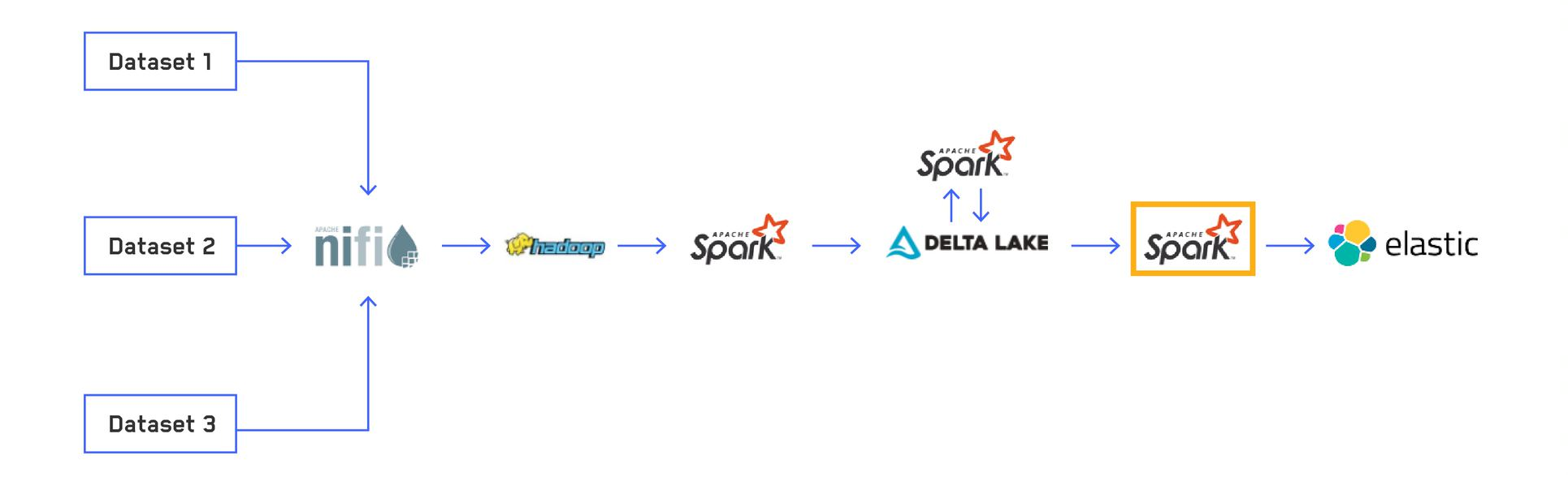
Editor’s note: This is the fourth and final post in a series titled, “Scalable and Dynamic Data Pipelines.” This series details how we at Maxar have integrated open-source software to create an efficient and scalable pipeline to quickly process extremely large datasets to enable users to ask and answer complex questions at scale. Read Part 1 of this blog series, which provides an overview of one of Maxar’s data pipeline processes; Part 2, which explains how and why we use Delta Lake; and Part 3, which describes how we use Delta Lake to optimize our file sizes.
The final step in our current Extract, Transform and Load (ETL) pipeline involves indexing the data into Elasticsearch, a distributed, free and open search and analytics engine for all types of data. We use Elasticsearch as our main interface for interacting with data from our custom applications. Elasticsearch is incredibly powerful and versatile for searching data, allowing us to run queries on over 100 terabytes (TB) of data in real time. We use the Elasticsearch-Hadoop library to index data from our Delta Lake tables through an Apache Spark™ structured streaming application. As of now, Elasticsearch-Hadoop doesn't support Spark 3, so we had to build our own custom version to support our Spark 3 pipelines. In this blog post, we will look at how our Elasticsearch cluster has evolved to suit our needs and the tips and tricks we have for indexing hundreds of billions of rows of data.
Our cluster evolution
As mentioned in Part 1 of this blog series, my team at Maxar runs on hardware that includes both hard disk drives (HDD) and non-volatile memory express drives (NVMe). Initially we took advantage of this by running two separate Elasticsearch clusters, one with the HDD as the backing store and one with the NVMe drives as the backing store. With this, we could index our small datasets onto the fast NVMe and reserve the HDD-backed cluster for our larger datasets.
This worked well for us until we really started trying to index a large amount of data onto our HDD-backed cluster. We found several ways to improve this throughput, but indexing requires a lot of random writes, and hard drives don't like random writes. The highest indexing rate we could reliably and consistently achieve without crashing the cluster was roughly 500,000 records per second, which averaged out to roughly 2,500 records per second per node. While this speed was adequate to start exploiting our data, it took nearly 24 hours to index a month's worth of data for some of our datasets. As we learned more about the data, we had to reindex based on our new knowledge, and this became an incredibly painful process. Additionally, we also run an Apache Hadoop® cluster on our nodes, and when we had Spark jobs running that were reading or writing a lot of data from the hard drives, the indexing rate dropped significantly. We knew this approach to using our HDD wasn't going to work for us in the long run.
Purely using the NVMe drives wasn’t an option either, as many of our datasets require access to the full corpus of data rather than just the most recent data, and these datasets don't fit entirely on the NVMe. We needed a way to index onto the NVMe and then move completed indices to the HDD. The snapshot and restore capability with Elasticsearch allowed us to do that with our separate cluster setup. We could index onto our NVMe cluster, snapshot to our distributed file system and then restore that snapshot into our HDD cluster. This worked well for us, and we were able to index around 350 TB of data over the course of a couple weeks. It worked so well in fact that we soon started running out of heap!
The good old JVM heap
At the time, we were running Elasticsearch version 6.7. Elasticsearch requires a certain amount of heap, memory allocated to the Java Virtual Machine (JVM), for all the data you have indexed, as it keeps information about disk locations of indices in memory. Once we approached about 2 TB of indexed data per node, we noticed our average heap usage rising above 90%. After doing some research, we found that more recent versions of Elasticsearch significantly decrease the amount of heap required for the same amount of data. See this blog post for a great explanation of these updates. We knew we had to prioritize upgrading our cluster if we wanted Elasticsearch to be able to handle this much data.
Upgrading and the hybrid-realization
Luckily, since we started with version 6.7, we didn't have to reindex any of our data, as Elasticsearch only supports reading one previous major version's worth of data. It took us some time to ensure our applications that interacted with Elasticsearch version 6.7 could work with version 7 too. The biggest required change was dealing with the new format of the total hit count. Once we were confident in our application updates, we rolling-upgraded our cluster to version 6.8, as it was required to update to this latest minor version before being able to rolling-upgrade to the current version, 7.8. After some slight hiccups along the way, we successfully upgraded our cluster, and our average heap usage immediately dropped to 50-60%.
While researching upgrading our cluster, we also stumbled across this blog post describing how to run a hybrid hot-warm cluster architecture, which allows hot data (data likely to be accessed frequently) to be stored on a node backed by NVMe and warm data (less frequently accessed but still relevant data) to be stored on a node backed by HDD on the same machine. We couldn't believe we hadn't come across or thought about doing this before, and it was clearly the exact fit for our situation. We deployed a second Elasticsearch instance on each node using the NVMe as the backing store, connecting to the original HDD-backed cluster. This allowed us to cut out the snapshot restore and simply use Elasticsearch's attribute-based routing allocation to index onto the NVMe and then simply relocate the shards onto the HDDs once we were done adding to each index.
Lessons learned along the way
With our updated cluster and NVMe usage, we can easily sustain an indexing rate of nearly 5 million records per second (averaging closer to 25,000 records per second per node). While we can probably find ways to improve this even further, it's plenty to meet our current needs to process backlogs of data and keep up with our daily feeds.
Once we are done adding new data to an index from a large dataset, typically in month-interval time-based indices, we force merge it down to one segment and then migrate it to the hard disks. Recently, there have been discussions that force merging to one segment isn't always ideal, but we believe it still holds true as the best case for hard drives as it reduces the number of random reads required to search.
Here are some lessons we learned and techniques we developed in addition to the standard tuning guides during our use of Elasticsearch:
Batch size
When we were still experimenting with indexing onto hard drives, we found that batch size made a huge difference for indexing rate. This made sense as the more data a single node could process at once, the more data could be written sequentially at once to the transaction log. We tested up to around a batch size of 80 megabytes (MB) and maxed out our indexing rate at around 100 running cores. The batch size had much less effect when indexing onto the NVMe, which makes sense as sequential writes are less of an issue. It can handle many more cores as well, and we've managed to scale up to 1,000 running cores to reach our 5 million documents per second sustained indexing rate. We also observed some heap usage and garbage collecting issues increasing the batch size significantly, though upgrading to Elasticsearch 7 has virtually eliminated our heap issues.
Strict mappings
One of the simplest things you can do to increase throughput and decrease storage size is strictly define your mappings. Elasticsearch has several built-in data types, including several options for each of these. It will infer a mapping for you if you don't provide one, but this inferred mapping can be much broader than you need. For example, the default mapping for a string-based column is two-fold: map it as a text type, which tokenizes content and is designed for long blocks of text, as well as keyword type if it's below 256 characters. The keyword type is designed for shorter, single value categorical data. Since a lot of the data we deal with is this categorical type of data, we can improve things by explicitly stating that these fields are only a keyword type and don't also get analyzed by the text analyzer.
While a good start, we can also improve on this further for keyword and numeric fields. For these types of data, Elasticsearch stores three main copies of each field:
- Source: The original raw data that Elasticsearch indexes. This is what's returned in the
_sourcefield for search results, in the same form it was sent to Elasticsearch - Index: The analyzed or normalized value that is used for searching the document and is not returned in any results.
- Docvalue: The analyzed or normalized value stored in a column-oriented format that is used for sorting and aggregations. This value is returned from aggregations and can be retrieved using the
docvalue_fieldsquery parameter via the Search API.
Each of these can be disabled for a certain field to conserve space and indexing time if they are known not to be needed. For example, a certain field might be useful for searching, but we know we will never run an aggregation on it. In that case, we can set doc_values to false in the mapping for that field. Other fields you might not even want to make searchable, you simply want them returned in the results. In this case, you can set enabled to false in the mapping. There are several other mapping parameters that can be customized, and for large datasets you really need to take care designing your field mappings.
Pre-sorting by shard
Related to the sequential write improvement of the larger batch size, we investigated ways of further increasing the amount of data processed by each node at once. Although a large batch size improves the size processed per transaction per node, that batch size still will be split up between possibly every shard in the index. Elasticsearch uses the document ID given (or if one isn't given, it creates one), hashes it and uses that to determine which shard the document belongs to. As we set the document ID explicitly for deduplication purposes, we were able to take advantage of this to essentially pre-sort our documents based on the destination shard.
The logic for generating the shard ID for a document can be found in org.elasticsearch.cluster.routing.OperationRouting, which makes use of a Murmur3 hash function wrapper defined in org.elasticsearch.cluster.routing.Murmur3HashFunction. We don't use any partitioning or custom routing settings, so the logic essentially boils down to
shard = murmur3(document_id) % number_of_shards
Because we operate in a fully Python environment, we chose to implement Elasticsearch's custom murmur3 wrapper as a Pandas user-defined function (UDF) rather than having to maintain a separate Java-based UDF. The overhead of using a Python-based UDF wasn't much of an issue for us, as Elasticsearch was still the main bottleneck in the process. Originally, we did a full repartitioning based on the shard number, but found the full shuffle generated too much overhead to make it worth it. We found that we could still get huge improvements doing a local sort. Assuming you want month-based indices, you have a DataFrame with a timestamp column called timestamp and a column holding the Elasticsearch document ID called document_id, the basic logic we use is:
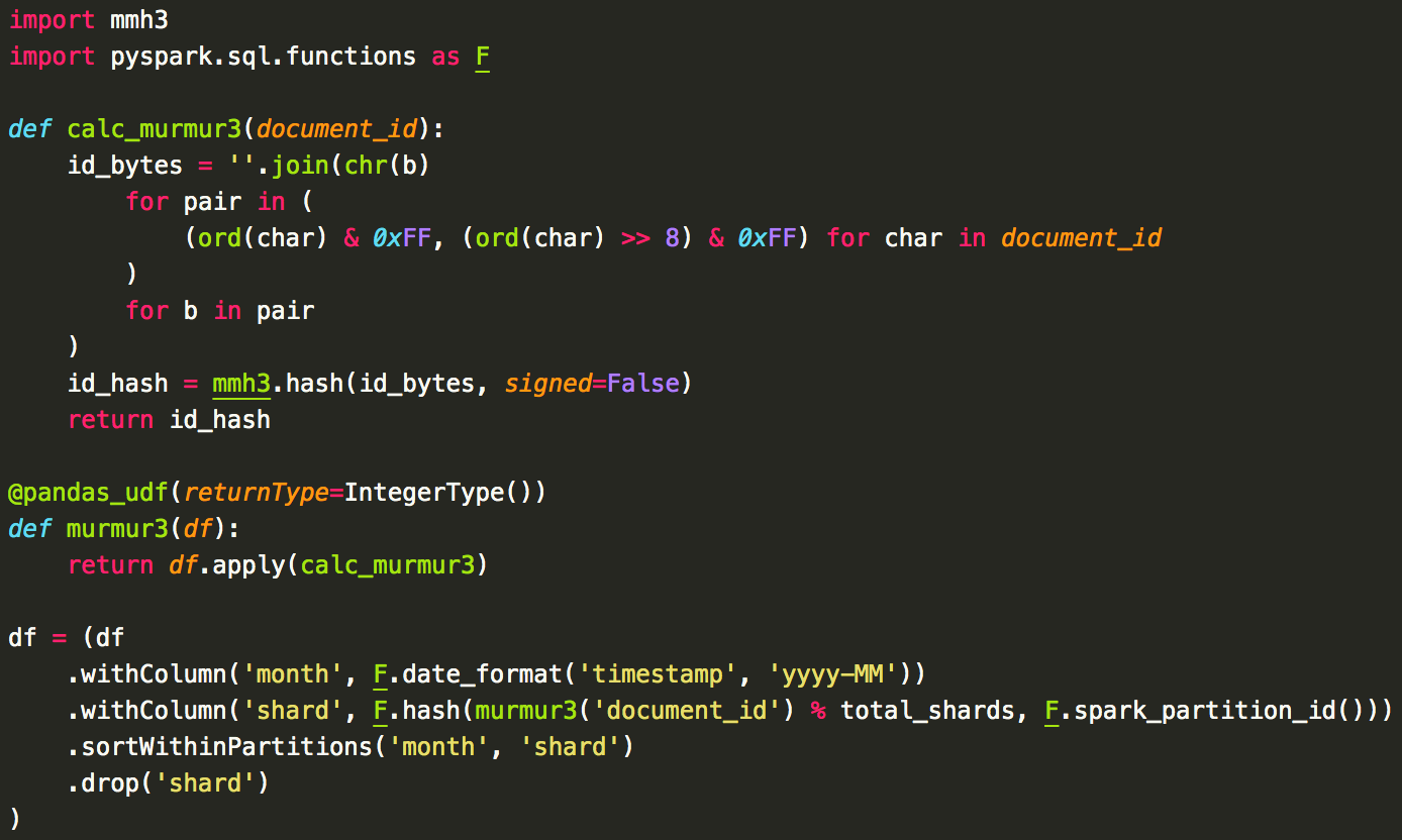
There are a couple things to note here. First, because each index has its own set of shards, we sort by the month in addition to the shard number. Second, we include the partition ID in our shard column calculation. Before we had this, we observed that eventually each Spark partition would get in-sync. Since each partition has the same ordering of the shards, eventually all cores would be attempting to index documents in shard 1, then shard 2, then shard 3, etc. and our throughput dropped drastically. By adding in the partition ID, this ensures that, for example, partition 1 will index documents on shard 5, then shard 1, then shard 3, etc. and partition 2 will index documents on shard 2, then shard 1, then shard 5, etc. preventing different partitions from syncing up.
It's also worth noting that while we sort based on shard number, we currently don't have a method for sending these documents directly to the node holding this shard. This would take constantly querying the state of the indexing and keeping track of where all shards are and would be a complex addition to the Elasticsearch-Hadoop library. Rather, our bulk requests will get sent to any Elasticsearch node, and that node will do its normal determination routing each document to the appropriate node. It just so happens that all that bulk request will then be routed to one or a small number of nodes.
With this pre-sorting, we noticed an incredible throughput increase when indexing on our hard drives. Unfortunately, we still ran into dramatic drops when the disks were also being used for other jobs we had running. When switching to only index on our NVMe nodes, we found that keeping the pre-sorting still allowed us to have a slightly higher and more consistent throughput, so we still use this approach.
Conclusion
Here we looked at the final step of our current data processing pipeline. We started with several raw datasets in various formats, standardized and normalized them into a common format of Delta Lake tables, optimized our tables for better batch query performance, and finally indexed the data into Elasticsearch. This is all being constantly streamed to expose data to end users in as little as a few minutes.
In the future, we can easily add new processes, such as streaming our data to a distributed graph database. Ultimately, this data pipeline process allows our end users can interact with hundreds of terabytes of data to gain the mission-critical insights.
Apache, the Apache feather logo, Apache Hadoop® , Apache Spark™, Apache NiFi™ and the corresponding project logos are trademarks of The Apache Software Foundation. Delta Lake and the Delta Lake logo are trademarks of LF Projects, LLC.