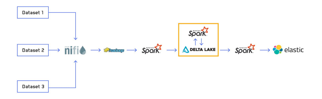
Editor’s note: This is the third post in a series titled, “Scalable and Dynamic Data Pipelines.” This series will detail how we at Maxar have integrated open-source software to create an efficient and scalable pipeline to quickly process extremely large datasets to enable users to ask and answer complex questions at scale. Read Part 1 of this blog series, which provides an overview of one of Maxar’s data pipeline processes, and Part 2, which describes how and why we use Delta Lake.
If you’ve read Part 1 and Part 2 in this blog series, you’ll be up to speed on the process I’m writing about. If you haven’t read it, here’s the short version: My team at Maxar is responsible for sorting through massive, disparate datasets to find mission-critical insights for our customers. This series is about the data processing pipeline we built to get that job done–and right now, we have our data in a nice column-oriented file format. So, we must be ready to run our complex analytics, right? While users can start running queries right away, they may find that simple actions such as counting records take longer than expected. This is because one of the byproducts of an Apache SparkTM streaming application is a lot of small files, and small files are very inefficient to read. Let's look at why that happens and how we get around this issue.
Why does Spark create small files?
To understand this, you first must understand the concept of partitions in Spark. Unfortunately, the term partition means two different things in the Spark world, and both are relevant to this problem. The first type of partitioning is a way to organize data in your file system to speed up queries that only need to look at a particular partition of data. An example would be partitioning time-series data by date. This allows you to filter by a date range and limit the files you read to those that fit your filter. Without partitioning, a date range filter would have to read all files of the table to find the matching rows. We'll call this table partitioning.
The second type of partitioning is how Spark distributes processing. A Spark Resilient Distributed Dataset (RDD), which underpins a Spark SQL DataFrame, is split into partitions. Each partition becomes a unit of work (task) that is assigned to a particular executor. In a simple case with no shuffling involved, a partition will load data from potentially multiple input files, perform its processing and write out its result to one or many files. We'll call this data partitioning.
On an unpartitioned table, a single data partition will output one file. However, when you have a partitioned table, you will get one output file for each unique table partition that is in each data partition. Let's say you have 10,000 rows of source data, load the data into a DataFrame with 100 data partitions and partition the output by a column that has 100 unique values. In an unpartitioned table, 100 data partitions mean you'll end up with at most 100 target files (ignoring settings like maxRecordsPerFile). However, in the worst case, each of your 100 data partitions could have rows with each of the 100 table partitions, meaning you'll end up with 10,000 target files, one with each row of data. This is clearly not an optimal solution, since we know a lot of small files does not perform well.

The diagram above illustrates how many small files can be generated from few source files. In this case, processing three source files result in nine output files.
Our optimization process
We tested out several methods for optimizing our file sizes and finally settled on post-processing our Delta Lake tables to minimize latency downstream and achieve the most consistent file sizes. Some other methods we attempted along the way are described later in this blog post.
The Delta Lake documentation clearly lays out how you can rewrite data after initial processing while indicating that you are not changing the data. This allows downstream processes streaming from your table to not register any changes. This can be done per table partition, letting you compact each table partition of many files into a partition of few files. The documentation only shows examples of repartitioning to a set number of data partitions, but it is hard to find a single value that best optimizes every table partition. You may be able to use metadata about the loaded DataFrame to determine the total file size and use that to find the right number to repartition to, but we found a more straightforward approach that avoids any kind of shuffle altogether. It relies on three key Spark settings:
spark.default.parallelism=1
This is the setting I least understand, but I found it had to be set to 1 to ensure maximum file size. It defaults to the number of cores you are running with and it's used as a kind of minimum amount of parallelism to use. If you have a partition that has total data less than your target file size, you may end up with more than one file if this is not set to 1 explicitly.
spark.sql.files.maxPartitionBytes=<target file size>
This setting determines how much data Spark will load into a single data partition. The default value for this is 128 mebibytes (MiB). So, if you have one splitable file that is 1 gibibyte (GiB) large, you'll end up with roughly 8 data partitions. However, if you have one non-splitable file (gzip compressed for example), you'll only have one data partition since there's no way to split it up. On the flip side, if you have 16 64 MiB files, you will also end up with around 8 (or slightly more due to the next setting) data partitions, as Spark will lump multiple files into a single data partition to try to reach the maximum bytes per partition.
Remember that Spark will create one output file per table partition in each data partition. If we operate on one table partition at a time, then what we effectively get is one file per data partition, and we can control how much data gets loaded into that data partition using this setting. This means if we ideally want 1 GiB files, we can set spark.sql.files.maxPartitionBytes=1073741824, and Spark will try to load up to 1 GiB worth of data into each data partition. Then when we write this data back out, we will end up with close to 1 GiB-sized files.
spark.sql.files.openCostInBytes=1
With just the other settings above, you will find that table partitions that already have relatively larger files will be rewritten in sizes close to your ideal size. However, if you have a table partition with many small files, your resulting file sizes will be much smaller. This is due to the openCostInBytes setting. What this essentially does is make small files appear to be larger. It's called an open cost because it takes longer to read 1 MiB each from two different data nodes than it does to read 2 MiBs sequentially from a single data node. This is due to various reasons like creating a connection to a new node and sequential disk access.
The default value for this setting is 4 MiB. This means that Spark will add 4 MiB to the size of all input files when calculating how to create data partitions. When running typical queries, this comes in handy by spreading out the work into more tasks. For the purposes of compacting files, however, we would rather trade off the longer time collecting all the small files to write all that data into consistently larger files. So, by setting this to a small value like 1, we essentially eliminate the open cost and let Spark pack as many small files as it can into a single data partition until it hits the maxPartitionBytes cap.
While 0 seems like the obvious setting for this to completely turn the open cost off, we ran into weird errors in Spark when trying it initially. In certain places various values, including the open cost, are used as a step value in a loop in Scala and trying to step by 0 throws an error and fails. We didn't track down what the actual other circumstances that led to that error were, as it happened rarely, and instead opted to just set this value to 1 and achieve nearly the same behavior.
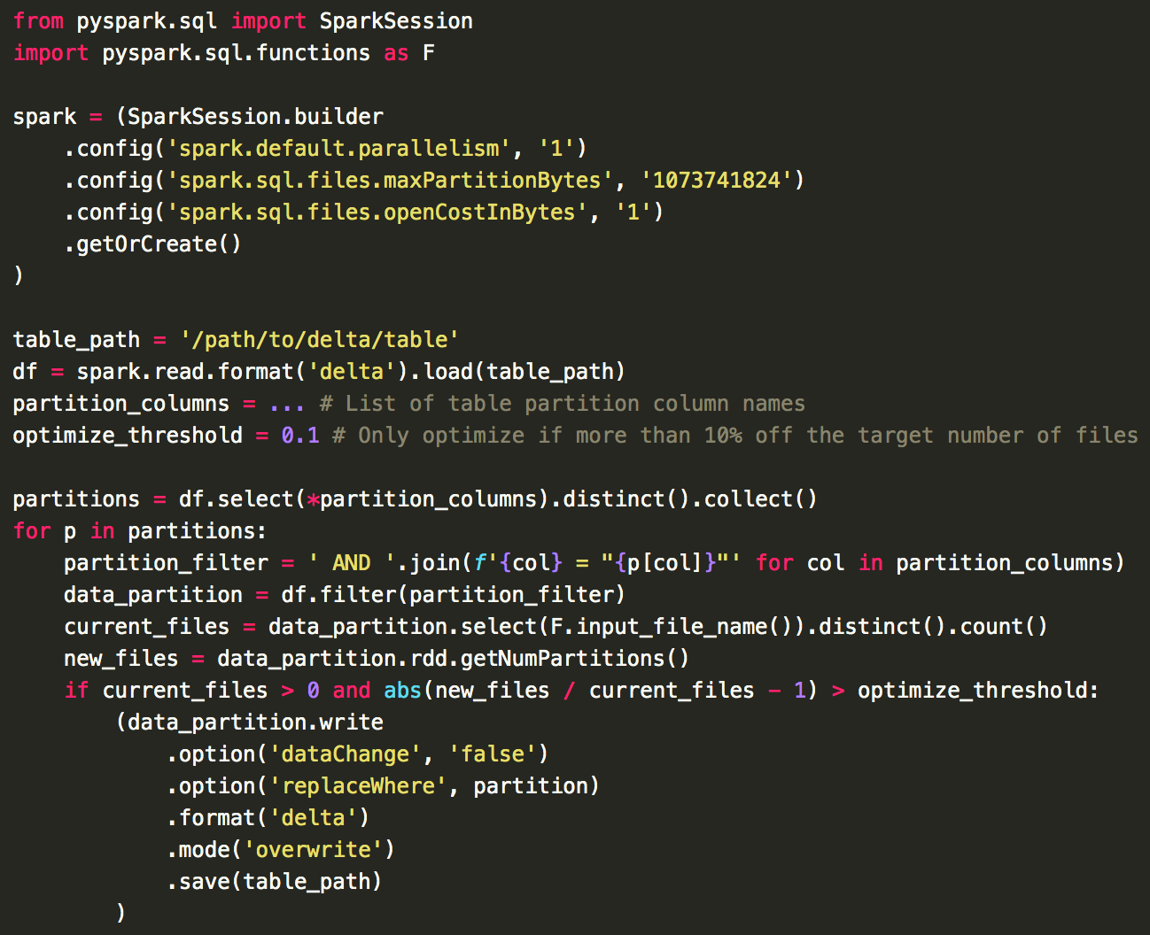
Calculating if a partition needs to be optimized
Because we partition our tables using timestamps within the data, we could receive new data going to any existing partition. When we optimize our tables, we need to check if any of our existing table partitions needs the optimization to be run. We do this by finding the difference between the number of existing files and the number of files that would be written out if optimized. If this difference is greater than our chosen threshold, then we run the optimization on that table partition, and if not, we skip it and move on. This threshold may need to be tweaked for different tables and still isn't a perfect system, but it works fairly well and avoids constantly rewriting the same data every time the optimization is run. The method we use to calculate this can be seen in this bare-minimum example code:
Alternative solutions
It took a few iterations to get to our current optimization technique. Here are the methods we tried and eliminated along the way.
Repartition by the table partition column
The first choice for increasing file size and decreasing file count is to repartition by the partition column before writing out the data. This does a great job preventing the small file problem, but it does it too well. What you end up with instead is one output file per table partition for each batch of data. For example, if you have five table partitions and you load five gigabytes (GB) of data evenly distributed across your output table partitions, repartitioning before writing should leave you with five 1 GB files, one in each table partition. However, if you load five terabytes (TB) instead, you'd end up with five 1 TB files. Obviously, it would take a long time to write a single 1 TB file (instead of distributing that across writing ~1000 one GB files), but it also isn't optimal for reading and analytics.
The solution to the large file problem is the spark.sql.files.maxRecordsPerFile setting mentioned above. This lets you tell Spark the maximum number of rows that can be in one output file. The problem with this is that it's a very hands-on process to find the correct number of rows that leaves you with your desired target file size. Additionally, it will be different for each dataset you work with and could change as you add or remove fields from your dataset. No matter how you approach this method, the shuffle also increases the latency to when the data is available to any downstream processes, so we kept searching for a better approach.
Rewriting data post-processing
With no ideal way to optimize file sizes before the initial write, we investigated ways to optimize files after the fact. We knew this would allow us to minimize the latency to when data is available downstream and allow us to better reach an optimal file size for the full dataset analytics we need to run.
Initially we worked with the built-in parquet output format in Spark. Its simplicity was very appealing, but it lacked the functionality we required, with no way to rewrite data without downstream processes seeing this as new data. We needed to find a Spark format with better metadata handling, which is what led us to the recently open-sourced Delta Lake.
Conclusion
What we have is a general-purpose solution that works on nearly any data set. While it doesn't achieve exact target file sizes, it comes pretty close. It only requires one heuristic (the optimized threshold) and avoids shuffling the data. We get much faster query execution compared to the initial output of our streaming applications, and we avoid overloading the name node with too many small files. In the final part of this series, we will examine the last step in our data processing pipeline: indexing to Elasticsearch.
Apache, the Apache feather logo, Apache Hadoop® , Apache Spark™, Apache NiFi™ and the corresponding project logos are trademarks of The Apache Software Foundation. Delta Lake and the Delta Lake logo are trademarks of LF Projects, LLC.