Blog

Editor’s note: This is the second post in a series titled, “Scalable and Dynamic Data Pipelines.” This series will detail how we at Maxar have integrated open-source software to create an efficient and scalable pipeline to quickly process extremely large datasets to enable users to ask and answer complex questions at scale. Read Part 1 of this blog series, which provides an overview of Maxar’s data pipelines process.

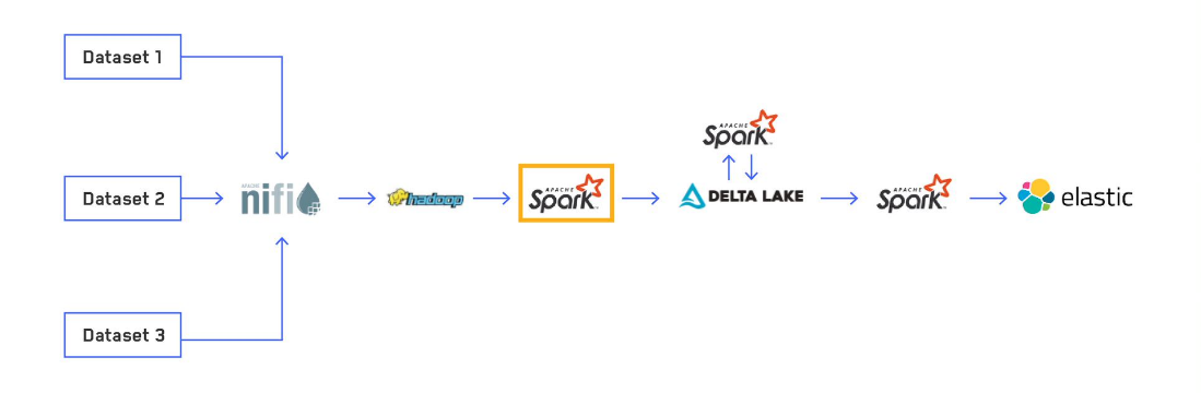
My team at Maxar routinely ingests large amounts of non-imagery based, geo-temporal data to provide mission critical insights for customers. The first core stage of our Extract, Transform and Load (ETL) data pipeline is using an Apache Spark^TM structured streaming application to load the raw data, apply common transformations and enrichments and write the data out to a Delta Lake table. We created our own Python library to abstract out as much of the common logic and boilerplate code as possible for creating production-ready Spark applications and centralizing the logic for normalizations and enrichments. In this post, we explore how we implemented this process and some of the difficulties we overcame.

Why Python

We implement our data processing using PySpark for a couple reasons:

• Most of the team’s developers have a stronger background in Python than in Java (and next to no background in Scala).
• Python is the go-to language for performing data analysis. Using a common language between our pipelines and our end users allows for streamlined collaboration.

The great thing about using PySpark with Spark SQL is that you don't sacrifice performance compared to natively using Scala, so long as you don't use user-defined functions (UDF). The Python DataFrame API is simply a wrapper around the Scala DataFrame API that constructs a logical plan of all the operations you specify. No processing happens until you do an output operation (show, collect, write, etc.), and at that point, your logical plan goes through Spark SQL's Catalyst optimizer which generates Java bytecode to run your operations.

Using a UDF written in Python can significantly slow your processing down, however. Spark must serialize every row, send it to the Python process, run your Python code and then deserialize back to Java. This can be improved using Pandas UDFs that use Apache Arrow for more efficient data transfer between processes. Still, we try to limit our use of Python UDFs as much as possible, as it will slow things down to some extent regardless. For the cases we are forced to write complex custom code, we have a separate library of UDFs written in Java that we use in our PySpark code.

Why Delta Lake OSS

When we initially started using Spark for our ETL process, we were only focused on getting the raw data into Elasticsearch, as that was our main place to expose data to users. Along the way, we played around with writing out our processed data to parquet files. We knew we would need to have our data in a format suited for more complex analytics, and parquet seemed to be the standard column-oriented file format for Spark. However, when experimenting writing out to parquet, we realized how many small files a streaming pipeline generates. The native Spark streaming sink doesn't have a way to optimize file sizes (beyond certain methods involving the maxRecordsPerFile option), which was a nonstarter for trying to use this in production.

We stumbled across Delta Lake, which was a Databricks-specific format but recently was open sourced as Delta Lake OSS. It provides numerous benefits on top of a simple parquet table, but the main one to us was the ability to rewrite data within a partition without registering changes in an application streaming from that table. This enables us to stream data from our Delta Lake tables to Elasticsearch without having to recompute all our normalizations and enrichments from the raw data. Part 3 of this blog series will cover more details of our optimization and file compaction process.

Creating a new pipeline (the E in ETL)

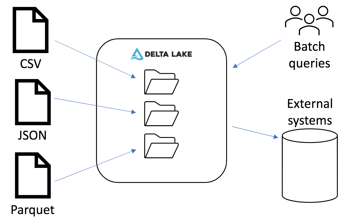
Data is messy. We receive datasets in all kinds of file formats and structures. The first step in creating a new pipeline is getting some familiarization with how to load that data format and learn what fields are in the dataset. This usually starts with reading the data in as a Spark DataFrame and letting it try to infer the schema. In cases of CSVs without a header, we need to determine the appropriate column names for the fields. JSON files have field names baked in, which simplifies some of the process. In the best-case scenario, Spark will be able to determine the correct schema without any conflicts. We will look at some hurdles we have run into trying to infer schemas later, but if things work successfully, we pull out the schema of a DataFrame df in JSON format with

print(df.schema.json())

We then save this in our Git repo along with our processing scripts. With the schema determined, we can load the dataset as a streaming DataFrame and continually process data as it comes in. However, before we get to that point, we must determine what normalization and enrichments to apply based on the fields present in the dataset.

A note on inferring parquet schema

If you are working directly with parquet files as your raw data, make sure to use

option("mergeSchema", "true")

when reading it as a DataFrame so that the schema from all parquet files will be collected and merged. Otherwise, Spark will assume the schema of all the files is the same and only pick one or a few files to load the schema from, possibly leading to dropped fields.

Applying transformations (the T)

One of the core modules in our data processing library contains all the common transformations we apply across our datasets. We construct our processed data with four top-level structures: raw, metadata, derived and normalized.

raw

The datasets we receive are so varied that it's impossible to know all possible use cases for each field. To provide the most value to our end users, we try to preserve the data in its raw form as much as possible. Within the raw struct, we keep the existing data structure and limit transformations to type coercion. For example, making sure float fields are typed as floats and not strings. Additionally, fields that are clearly a delimited list of values will be split into an array.

metadata

Metadata fields are for internal tracking and data provenance purposes. The main fields we store in here are the path of the raw file this row came from originally and the time it was ingested.

derived

These are enrichments that we can derive from the raw data that provide enough use to precompute rather than computing on the fly for analytics. The most common derivations we use are a master timestamp for the record (the best timestamp representing the record, possibly from several different timestamps within the record) and the country code for geolocated data. These provide value for basic partitioning and filtering.

normalized

Once again, data is messy. Different data sources can have the same type of field but formatted wildly different. Here we create a copy of a raw field with the same inner path but in a format we have chosen for normalizing that type of field. Common normalizations we perform are lowercasing and removing special characters.

Every additional field we add to our data comes with a storage cost, so the value being added must be carefully considered.

A note on nested structs in Spark

We make heavy use of structs in our Delta Tables. Since these are backed by Spark's built-in parquet file format, individual deeply nested columns can be loaded efficiently in certain circumstances. In the version of Spark we are using (3.0.2), loading individual nested columns will only read that column's data from disk for simple operations. Unfortunately, some queries like groupBy will still load the entire top-level struct from disk even when only using one nested column. There are currently ways you can get around this limitation (such as select fields before doing a groupBy), but many of these limitations have been addressed in the master branch and are now available in the latest minor release (3.1). When in doubt, you should always run an explain on your query to see what it will be doing. What's listed in the ReadSchema are the fields that will be physically read from disk for your query.

Writing to Delta Lake (the L)

The last step in ingesting data to Delta Lake tables is, well, writing to a Delta Lake table! This step is straightforward: Simply choose the output directory as well as checkpoint location for streaming DataFrames. We make this step extremely simple by taking care of many of these required options with our second core module.

Job library

The second main module of our data processing library is our job module, which encapsulates a lot of the common behaviors and settings around running a Spark application. Some of the core features we have added include:

• Support for adding default values for various common Spark properties (including the streaming trigger interval) and the ability to override them on the command line when launching applications
• Standardized checkpoint and output directory path determination based on the dataset name and version
• Wrapper around read/readStream/write/writeStream that enables one application to work with both streaming and batch modes based on a command line argument, letting us easily use batch mode for testing and streaming mode for production
• Creating a pidfile in the file system that is constantly monitored and shuts the Spark application down when deleted—the only way we have found to cleanly shut down a streaming Spark application

These features let us create production-ready applications while minimizing the duplicated code across datasets.

Real scenarios we have encountered

These are some examples of difficulties we have encountered when creating pipelines for new datasets and how we overcame them.

Schema inferencing errors

Several of the issues we have encountered involve inferring schema from both JSON files and parquet files. Some we could solve, and some forced us to ignore certain fields.

Mixed casing of field names in JSON

One instance we ran into happened when the JSON data we were working with had certain fields that were sometimes camelCase and sometimes all lowercase. Spark is generally case insensitive with field names but keeps the exact text when inferring fields from JSON. In this case, two separate field names were inferred in different files and when the case-insensitive schema was merged, there were duplicate field names, which causes an error to be thrown in Spark. We were able to get around this issue by setting spark.sql.caseSensitive=true when inferring the schema, finding the duplicates and deleting one of them. The schema then worked for both cases with case sensitivity turned back off (the default).

Changed parquet schema

Some data we receive comes already in parquet format. It's great receiving already strongly typed data, except when the data provider changes the schema unexpectedly. Two examples we ran into involved a boolean field in the data. Some of the files correctly had this as a boolean type, where other files had it as an integer type that was either 0 or 1. Spark crashed trying to infer the overall schema because boolean and integer are not compatible types. In the first instance, we were able to find a distinct point in time where the schema changed and could simply load data before that time one way and after another. In a second instance, the difference was randomly dispersed throughout the data, so we opted simply to ignore that column as it was determined not to be important. There's no obvious fix we have found for this case.

Heavily nested archives

One dataset we receive comes to us as a series of heavily nested combinations of .zip and .tar archives. While we typically extract archives in Apache NiFi^TM before writing to our file system, the number of nested files was so great that it would overwhelm our NameNode. Instead, because the overall dataset is relatively small (there are a lot of very tiny and diverse files), we opted to create our own custom Spark data source. It is based on the Spark built-in binary data source, recursively extracting any archive it comes across and returning the binary content of the leaf files as well as the filenames of all the archives along the way. From this point, we at least have the content of each file in a row and can continue with our custom processing. While this is not what Spark was designed for, and there are clearly limitations on the size of files that can be read, fitting this scenario into the rest of our standardized pipeline proved easier than designing a fully custom process for this dataset.

Conclusion

In this blog post, we examined our process for creating Delta Lake tables from diverse data sets. Delta Lake allows us to optimize file sizes for improving downstream query performance. Our custom library reduces boilerplate code across our applications and helps us establish standard transformations. Overall, by taking the time to process everything to a standard format, we have a better foundation for running large batch queries and streaming to external systems.

Apache, the Apache feather logo, Apache Hadoop® , Apache Spark™, Apache NiFi™ and the corresponding project logos are trademarks of The Apache Software Foundation. Delta Lake and the Delta Lake logo are trademarks of LF Projects, LLC.